This paper mainly focuses on using different methods to estimate covariance matrix and fixed income securities to maximize return and minimize risk for portfolio optimization and Index Replication. The methods would be based on our research in the field of, quantitative financial theory and statistics theories, which are Sample Covariance Matrix Estimation, Weighted Sample Covariance Matrix Estimation, and Shrinkage Estimation for Covariance Matrices.

We are developing filter methodologies for our datasets by splitting the data into high yield and low yield Investment grade bonds to explore in this project. The main purpose of this project is to provide an accurate risk measure, develop covariance matrix estimation methods and finally use our findings for fixed income portfolio construction decisions.

Key words: Covariance Matrix Estimation, Fixed Income Securities, Portfolio Optimization

I. Introduction

1.1 Background

Fixed income securities are debt instruments that deliver a fixed interest fee in exchange for some committed capital. They are not as volatile or dynamic as stocks but nonetheless fluctuate in value depending on market conditions. Building a portfolio or index replication composed of fixed income securities can be quite difficult, covariance matrix estimation is essential for index replication since it’s not feasible in the corporate bond market to purchase all the bonds in an index. In addition, covariance matrix is essential for portfolio manager to establish portfolio and base on Modern Portfolio Theory in 1959, mean-variance methods which is the sample covariance methods have issues when the assets are increased. Besides, the Modern portfolio theory are based on the assets allocation of equites instead of Fixed income. As a result, covariance matrix estimation is important not only for the portfolio but also the co-movement of the assets. Moreover, covariance matrix could help portfolio manager quantify the risk and find a better portfolio optimization. Therefore, in this paper, we will implement Sample Covariance Matrix Estimation, Weighted Sample Covariance Matrix Estimation, and Shrinkage Estimation for Covariance Matrices and test the results using Mean Absolute Error (MAE), Roots Mean Square Error (RMSE) to estimate the model and find out which method provided better solutions for building portfolio or reduce the risk of portfolio.

Consequently, this paper is organized as follows. In this section, we give an Introduction, research objective, problem statement and the definition for whole project. In section II, we will focus on Data Acquisition, which is our data analysis and how each observation means. In addition, we will provide a short idea on each observation. In section III we will focus on the analytics and Algorithms which will be an idea of what methods we will use for this project and mathematics, Statistic theory for this project. In section IV, we will deliver a visualization for this project which is to visualize result for the project. The conclusion and summary will be in section V and finally for Future research, we will provide our recommendation and areas of focus on section VI.

1.2 Research

Portfolio optimization is currently a multi-step process where inputs are focused and then sent to the optimizer (Ledoit & Wolf, 2003). The optimizer assumes the forecasted values are accurate and generates an “optimal” solution. For Index Replication, the quality of replication is measured by tracking error (TE) defined as the standard deviation of the difference between the return on the portfolio and that of the benchmark (Martellini, Priaulet, & Priaulet, 2003). A key component for both of these processes is the covariance matrix between securities. Our principal task in this project is to estimate the covariance matrix of the returns of fixed income securities in order to find an optimal allocation of assets that minimizes risk, maximizes returns and replicate the returns of an index. Since there is a lakh of literature in covariance matrix for fixed income securities our project has focused on exhaustive research into available methods and developing an implementation and testing framework for some of the simpler methods (Neffelli & Resta, 2018).

1.3 Project Objectives

● Literature review of covariance matrix estimation in fixed income.

● Conduct an exploratory data analysis on the acquired dataset of fixed income securities and their relationships to each other.

● Create objective performance metrics, baselines, and validation procedures using inputs from domain experts.

● Explore methodologies to estimate the covariance matrix of fixed income portfolio returns.

● Visualize results and recommend a final methodology.

1.4 Problem Space

The covariance matrix estimation is widely used for analyzing the financial data, for example, the stocks, options, risk measure etc. However, it will cause estimation issues if we apply the covariance matrix to the fixed income directly, since the result may not be accurate when the number of observations of each asset is larger than the number of assets we have in the data. We need to find a way to reduce the number of observations of each asset in the dataset. Secondly, we need to provide a better solution to reduce error on covariance matrix and which could provide a better construction of portfolio. Finally, provide accurate risk measure on portfolio.

1.5 Primary User Story

Our Projects main task is to build covariance matrix estimation using Sample Covariance Matrix Estimation, Weighted Sample Covariance Matrix Estimation, and Shrinkage Estimation for Covariance Matrices to analyze the fixed income portfolio in order to minimize the risk and maximum the return. If we can find a way to apply the covariance matrix estimation method to the fixed income securities, Companies like Principal Finance Group can reduce their costs to third parties by utilizing the methods developed in this project.

1.6 Solution Space

The 3 methods applied to create models are

1. Sample Covariance Matrix Estimation

(Martellini, Priaulet, & Priaulet, 2003) [1]

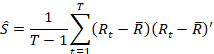
Where T is the sample size, n is the number of bonds in the portfolio, and the N – vector of the bond returns in the period t and the N-vector of the average of these returns over time. However, the sample covariance matrix has too many parameters and has resulted in large errors.

2. Weighted Sample Covariance Matrix Estimation

(Martellini, Priaulet, & Priaulet, 2003) [1]

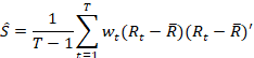
Whereis the weight for the observation at time t.

This estimation is related to time, therefore it is good for time tracking and narrow down errors. Also, allows us to assign a decaying weight to observations from further back in time.

3. Shrinkage Estimation

(Ledoit & Wolf, 2003; Demiguel, Martin-Utrera, & Nogales, 2011) [2][3]

The sample covariance matrix has many advantages. For example, it is easy to compute, and it is unbiased. However, a sample covariance matrix may contain a lot of estimation error especially when the number of observations of each asset is smaller than the total number of assets in a portfolio. This is the reason why we need to come up with a new method to compute the covariance matrix in order to reduce the estimation error.

The basic idea of shrinkage estimation is that, suppose we have a sample covariance matrix, denoted by S and a “highly structured” estimator, say, F. We want to find a compromise between S and F by computing a convex linear combination , where is a small real number between 0 and 1. In other words, the “highly structured” estimator F is our “target” matrix and we want to shrink our sample covariance matrix toward to the “target” matrix, F.

According to the convex linear combination , we can see when , the “shrunk covariance matrix” is the same as the sample covariance matrix, S; and when , the “shrunk covariance matrix” is just the “target” matrix, F. How to define the “target” matrix, F and the “optimal” value of are the key points of Shrinkage Estimation and conducting the shrunk covariance matrix.

In our project, the shrinkage estimation shrinks the sample covariance matrix towards a so-called global average that theoretically represents a true estimate of the covariance matrix by using R package called “tawny”. In other words, the global average of our sample covariance matrix is the “target” matrix, F. The value of is calculated by the “tawny” package in R automatically.

1.7 Product Vision - Sample scenarios

Assets management company or portfolio manager use Modern Portfolio Theory (MPT) that Markowitz establish in 1952 to build a mutual funds (Miller, 2019). However, during the time that Markowitz established the model, it did not deal with problems faced today, which is the High dimensional financial data (Karoui, 2010).

The theory during 1952 does not work well in real world situation. Mainly because in quantitative finance field, the problem of modern portfolio theory topic is widely been discussed (Elton & Gruber, 1997).

This problem affects the accuracy of portfolio construction and increase the risk of portfolio. The Modern Portfolio Theory is based on mean-variance matrix which is the sample covariance matrix. Second, the covariance matrix is ultimately used to optimize different securities of a portfolio.

Therefore, the risk and return have a trade-off issues in the Modern portfolio theory. In addition, the mean variance matrix has an issue with the size of the matrix. As a result, when the assets of portfolio are increase the risk of the portfolio will be increase.

Therefore, Principal Financial wants to estimate the Covariance to facilitate optimization to minimize the cost of transaction and calculate risks when selecting securities. However, unlike equities, bonds are impacted by several factors and there has been less research on covariance matrix when it comes to fixed income securities. For example, the yield to maturity, the duration, the interest, credit rating, the coupon rate and so on will affect the price of bonds. Therefore, in fixed income, the Covariance Matrix is much harder to estimate as compared to equities. All in all, to reduce the error of covariance matrix and estimate the true matrix of fixed income is our primary goal.

1.8 Definition of Terms

1. Fixed income: Fixed income is a type of investment whose return is usually fixed or predictable and is paid at a regular frequency like annually, semi-annually, quarterly or monthly. (Chen, 2019)

2. Covariance Matrix: Is a matrix whose element in the i, j position is the covariance between the i-th and j-th elements of a random vector. (GRACE-MARTIN, 2018)

3. Weighted Sample Covariance Matrix: A weighted covariance allows you to apply a weight, or relative significance to each value comparison. Covariance comparisons with a higher value for their weight are considered as more significant when compared to the other value comparisons. (WeightedCov, n.d.)

4. Shrinkage Estimation: “Shrinkage is where extreme values in a sample are “shrunk” towards a central value, like the sample mean.” (Stephanie, 2016)

5. Modern Portfolio Theory (MPT): MPT is the theory on how risk-averse investors can construct portfolios to optimize or maximize expected return based on a given level of market risk, emphasizing that risk is an inherent part of higher reward (Chen, 2019)

II. Data Acquisition

2.1 Overview

The Principal Company provided us with two datasets with High Yield bonds and Investment Grade bonds. The length of time for each bond is different. At first, we believed we could use the variable of excess return to build the sample covariance matrix. However, we quickly realized that the sample covariance matrix cannot be used directly, a direct use can seriously affect the estimates of the mean and variance, resulting in large errors. Our objective of this project is to explore methods for estimating the covariance matrix between a collection of fixed income securities.

2.2 Field Descriptions

● US-HY - HIGH YIELD

● US-IG - INVESTMENT GRADE

● Accrued Interest (Type: numeric) – The interest on the bond that has accumulated since the principal investment.

● Amount Outstanding (Type: string) – The principal amount outstanding of a bond (a.k.a. notional amount).

● Class 1(Type: string) – Blanket bond type (typically, corporate, government, etc.)

● Class 2, 3, 4(Type: string) – More specific industry of bonds.

● Country (Type: string)– Country in which the bond was issued.

● Coupon (Type: numeric) - The annual interest payment that the bondholder receives from the bond's issue date until it matures.

● Currency (Type: string) – Monetary unit in which the bond is valued.

● CUSIP (Type: string) - An acronym that refers to Committee on Uniform Security Identification Procedures and the nine-digit, alphanumeric CUSIP numbers that are used to identify securities, including municipal bonds.

● Description (Type: string)– (Potentially) The holding company of the issuer of the bond.

● DTS (Type: numeric) – Duration Times Spread; a measure of risk.

● Excess Return (Type: numeric) – The percent increase in the security’s value above the risk-free fate of interest, since the last month.

● FX to Base (Type: numeric) – The relationship of the bond’s currency to USD.

● Index Rating (Type: numeric) – The bond’s credit rating.

● ISIN (Type: string)– International Securities Identification Number.

● Issue Date (Type: datetime) – The date a bond was issued.

● Issuer Name (Type: string) – The issuer of the bond.

● Market Value BOM (Type: numeric) – Market Value Beginning of Month; the raw market value of the bond at the beginning of the preceding month.

● Market Value % (Type: numeric) - The percentage of the index’s market value comprised by a bond.

● Maturity (Type: numeric) – Years remaining until the bond reaches maturity.

● Moody’s Rating (Type: numeric) – Bond credit rating from Moody’s.

● OAD (Type: numeric) – Option-Adjusted Duration; Approximates the degree of price sensitivity of a bond to changes in interest rates, adjusted for embedded options.

● OAS (Type: numeric) – Option-Adjusted Spread; The measurement of the spread of the bond and the risk-free rate of return, adjusted to account any embedded options.

● Price (Type: numeric) – The price an investor would have to pay at that point in time to purchase the bond.

● S&P Rating (Type: numeric) – Bond credit rating from Standard and Poor.

● Ticker (Type: string) - An abbreviation used to uniquely identify publicly traded securities.

● Total Return (Type: numeric) – The percent increase in the security’s value since the last month.

● Yield to Worst (YTW) (Type: numeric) – The lowest possible yield for the bond.

2.3 Data Context

Bonds are issued by governments and corporations when they want to raise money. By buying a bond, one is giving the issuer a loan, and they agree to pay back the face value of the loan on a specific date, and to pay periodic interest payments along the way, at certain intervals. Unlike stocks, bonds issued by companies provide no ownership rights. So, you don't necessarily benefit from the company's growth, but you won't see as much impact when the company isn't doing as well, either—as long as it still has the resources to stay current on its loans. Bonds, then, give two potential benefits when you hold them as part of your portfolio: They give you a stream of income, and they offset some of the volatility you might see from owning stocks.

Portfolio optimization is the process of finding the best portfolio by maximizing expected return and minimizing financial risk. In this project we are concentrating only on bonds. So typical we are trying to optimize the bonds considering different factors and try to get maximum return with least amount of risk. So as mentioned in the field description data gives all the factors for a bond portfolio optimization.

2.4 Data Quality Assessment

Completeness: Missing values contributed to our dataset requiring heavy cleaning in order to analyze effectively. We used the excess return to build our covariance matrix. While there was an abundance of null values in our dataset, we addressed the issue of completeness by removing null values of excess return that were largely incomplete. We also had to merge excess return datasets from different time periods for every bond before analysis.

Uniqueness: The uniqueness of our dataset is using Committee on Uniform Security Identification Procedures (CUSIP) to directly determine every single bond. Using Observation ‘issues date' for searching single bond was largely unsuccessful, although our data is time series data. There are different bond yields at the same time. Therefore, when we use the CUSIP variable to filter, it is easy to select the excess return status of the same bond in different time periods.

Accuracy: We believe our dataset to be extremely accurate based on historical excess return for each bond that occur every year. The dataset is provided by the Investment department of Principal Group.

Atomicity: The dataset has a medium level of atomicity. After initial reviews of the dataset we found a certain bond were collected before the bonds were issued, these findings lead us to examine the accuracy of the data and we found that the total return, excess return and market value are null. From this assessment we decided not to use this part of data for our assessment.

Conformity: The original data we received obtained relatively high conformity. All data fields were presented in the expected formats. For analysis purposes, a large part of initial data cleaning entailed transforming text attributes to usable numerical formats. We also utilized R, Python and excel to delete some null values and clear up summary of data in order to analyze further.

Overall quality: We thought the overall data quality was high. A large part of any data analytic project is data cleaning and exploration in order to analyze effectively. We believe the amount of time spent to understand and clean our data was in line with previous projects and that overall, we are grateful for the quality of the data we were able to obtain.

2.5 Other Data Sources

We use Barclays High-Yield Index, Barclays Investment Grade Index and Barclays High Yield Total Return Index. There are over 260k values in High Yield dataset, almost 600k values in Investment Grade dataset and near 30 observations in both datasets.

III. Analytics

Part I. Bond Selection method

We created a rating system in order to sample our data not only for High yield bonds but also for investment grade bonds. The basic idea is that, we summarized the High Yield Bond Index data. That is, we calculated the mean value of S&P Rating, Option-Adjusted Spread (OAS), Option-Adjusted Duration (OAD) and Yield to Worst (YTW) in Index data. Then, we calculated the mean value of S&P Rating, OAS, OAD and YTW for each bond. Then, we came up with the following rating system.

Rule	Point earned
Bond AVG.OAS < Index AVG.OAS	1
Bond AVG.OAS > Index AVG.OAS	0
Bond AVG.OAD < Index AVG.OAD	1
Bond AVG.OAD > Index AVG.OAD	0
Bond AVG.YTW < Index AVG.YTW	0
Bond AVG.YTW > Index AVG.YTW	1
Bond AVG.S&P Rating < Index AVG.S&P Rating	1
Bond AVG.S&P Rating > Index AVG.S&P Rating	0

Figure 1. Sampling method

After we apply the rating system, each bond will get point in 0 ~ 4 scale. A bond with higher rating point means that bond has more risk. For example, there are more than 500 High Yield bonds have full records from 2015 – 2018, and the rating distribution is below:

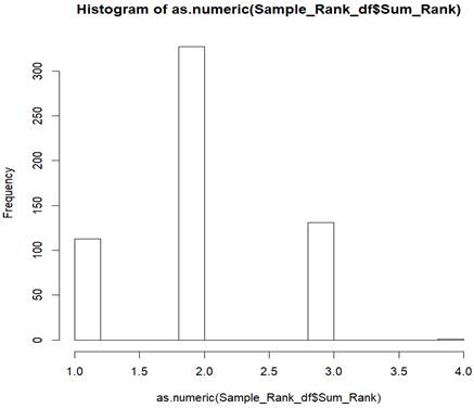
Figure 2. Distribution of each score

From the histogram plot, we can see that most of the bonds have two points. The ratio for number of bonds in those four rating groups is 113:327:131:1. Suppose we want to select 150 bonds according to the rating group, we will select 30 bonds from rating group 1, 86 bonds from rating group 2, 34 bonds from rating group 3 and 0 bond from rating group 4 (the ratio of the bonds we selected from four rating groups is approximately 113:327:131:1). This is the basic idea of our sample selection.

Part II. Empirical testing

We have two datasets which is High yield bonds and Investment grade Bonds. We tested all three methods on these two datasets. However, after the sampling we could only find 100 sufficient data in High yield bonds and 200 for investment grade bonds from the period 2011 to 2018. As a result, the test might have bias but still have certain reference value.

a. High Yield Bonds

Long term with information leaking

100 bonds selection for different time periods:

In our situation, we found out HY dataset only has 73 bonds in every month of each year from 2011-2018, so we split these years to 5 time groups, which are 2011 - 2013, 2012 - 2014, 2013 - 2015, 2014 – 2016 and 2015 - 2017, and then add other 27 bonds by applying our bonds selection method in each group so that 100 bonds can be assembled. For example, we selected 27 bonds which have full records between 2011 - 2014, but only chose the observations between 2011 - 2013 of those 27 bonds and added them to group one (2011 - 2013).

Therefore, we have 100 bonds in group one. For group two (group of 2012 - 2014), we applied the same sampling method. It contains the 73 bonds which have full records from 2011 to 2018, and we took 7 bonds which have full records from 2011 to 2014 in group one into group two. Then we selected another 20 bonds which have full records from 2012 to 2015, but only chose the observations between 2012 - 2014 and added them to group two.

Therefore, we have 100 bonds in group two. This way of selecting bonds will guarantee that there are 80% of bonds in group one that are also in group two. The same approach was used for the remaining groups. Our bond selection methods ensure 80% of bonds in group one is included in group two. However, this way of selecting bonds will cause information leakage.

Conduct the covariance matrices by applying different methods and test the performance

After we finished bonds selection for HY data, we did the covariance matrices by applying sample, weighted and shrinkage methods. Then we tested the performance for each method. Our performance testing method is to compute the Mean Absolute Error (MAE) between the estimated CVm and the true CVm. That is, we defined the true CVm as the sample CVm at time T + 1; for example, if we defined the time period of 2011 - 2013 as time T, the time period of 2012 - 2014 will be T + 1 then. Here are the performance testing results.

High Yield Bonds: Sample vs. Weight Sample vs. Shrinkage MAE Compare
TIME(T)	T+1	Sample MAE	Weighted MAE	Shrinkage MAE
2011-2013	2012-2014	5.666	2.854	5.835
2012-2014	2013-2015	2.628	2.531	2.526
2013-2015	2014-2016	4.290	4.086	4.277
2014-2016	2015-2017	4.444	5.289	4.443
2015-2017	2016-2018	4.824	3.670	4.739

Figure 3. 100 High yield bonds with information leaking MAE comparison

Short term without information leaking

In order to avoid the information leakage, we came up with another way to conduct the CVm for HY data. That is, we used the data from the time period of 2011 - 2013 to conduct the CVm by applying those three methods and defined the true CVm as the sample CVm of 2014 data; then we computed the MAE between them. We also used the data from time period 2015 - 2017 to conduct the CVm by applying those three methods and defined the true CVm as the sample CVm of 2018 data; then we computed the MAE between them. Here are the results:

High Yield Bonds: Sample vs. Weight Sample vs. Shrinkage MAE Compare
TIME(T)	T+1	Sample MAE	Weighted MAE	Shrinkage MAE
2011-2013	2014	6.684	3.852	6.654
2015-2017	2018	4.221	2.558	4.198

Figure 4. 100 High yield bonds without information leaking MAE comparison

b. Investment Grade Bonds

Long term with information leakage

200 bonds selection for different time period.

In this situation, there are more than 700 bonds which have full records between 2011 - 2018. We chose 200 bonds by applying our bond selection method and divided the observations of those 200 bonds into 5 time groups which are 2011 - 2013, 2012 - 2014, 2013 - 2015, 2014 - 2016 and 2015 - 2017. This way of selecting bonds will cause information leakage.

Conducted the covariance matrices by applying different methods and tested the performance. Here are the results:

Investment Grade: Sample vs. Weighted Sample vs. Shrinkage compare
TIME(T)	T+1	Sample MAE	Weighted MAE	Shrinkage MAE
2011-2013	2012-2014	1.981	0.986	1.813
2012-2014	2013-2015	0.682	0.298	0.646
2013-2015	2014-2016	0.773	0.782	0.772
2014-2016	2015-2017	0.112	0.390	0.151
2015-2017	2016-2018	0.223	0.421	0.234

Figure 5. 200 Investment grade bonds with information leaking MAE comparison

Short term without information leakage

In order to avoid the information leakage, we used the data from the time period of 2011 - 2013 to conduct the CVm by applying those three methods and defined the true CVm as the sample CVm of 2014 data; then we computed the MAE between them. We also used the data from time period of 2015 - 2017 to conduct the CVm by applying those three methods and defined the true CVm as the sample CVm of 2018 data; then we computed the MAE between them. Here are the performance testing results:

Investment Grade: Sample vs. Weighted Sample vs. Shrinkage MAE Compare
TIME(T)	T+1	Sample MAE	Weighted MAE	Shrinkage MAE
2011-2013	2014	2.944	1.959	2.779
2015-2017	2018	0.833	0.583	0.791

Figure 7. 200 Investment grade bonds without information leaking MAE comparison

IV. Visualization and Results

In this part, we show correlation plots and the MAE chart for the three estimation methods we used (Sample, Weighted and Shrinkage) in HY and IG datasets. Efficient Frontier is also displayed to demonstrate the portfolios.

a. High-Yield 100 bonds correlation plots

As we can see the color of each small box in the correlation plots, weighted CVm is lighter than the Sample CVm. The third one, which is shrinkage CVm seems like the color is close to light blue which means it reduce more correlations, however, due to the characteristic of shrinkage estimator, the result is too extreme. Therefore, Weighted CVm has a better performance than the other two methods in our analysis.

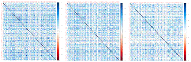
Figure 8. Correlation Plot for Sample, Shrinkage and Weighted-HY

b. Investment Grade 200 bonds correlation plots

Even though the graphs are too big to display, similar to High-Yield bonds, Investment Grade bonds have a same result. We also find out that performance of Weighted CVm is better.

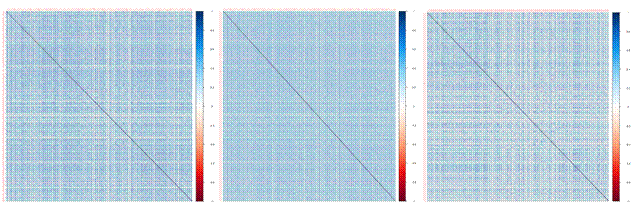
Figure 9. Correlation Plot for Sample, Shrinkage and Weighted-IG

c. MAE charts for HY dataset

On the left-hand side is the MAE chart for HY dataset with information leakage; on the right-hand side is the MAE chart for HY dataset without information leakage. We can see whether we have information leakage or not, the weighted covariance matrix always has a better performance since the MAE values are smaller than the other two methods based on our analytics results.

Figure 10. MAE Charts for HY

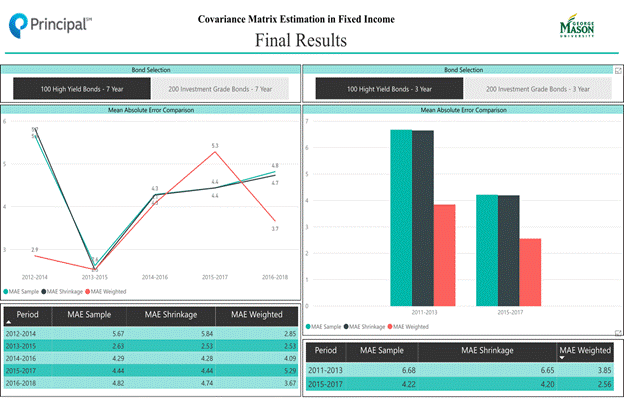
d. MAE charts for IG dataset

On the left-hand side is the MAE chart for IG dataset with information leakage; on the right-hand side is the MAE chart for IG dataset without information leakage. We can see whether we have information leakage or not, the weighted covariance matrix always has a better performance since the MAE values are smaller than the other two methods based on our analytics results.

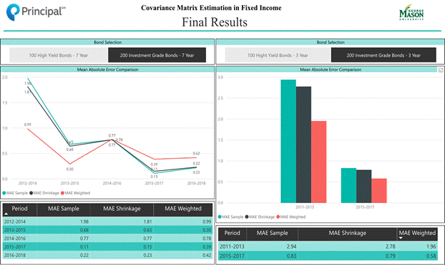
Figure 11. MAE Charts for HY

e. Efficient Frontier and Portfolios by 200 shrunk bonds (For future research)

The graph below shows that we could find the maximum return and minimum risk of the portfolio. However, in our case, after the test we could only use the Shrinkage Covariance matrix to build the Efficient frontier. The Sample covariance Matrix and weighted sample covariance could not build the Efficient frontier. The reason being, covariance matrix is affected by size, which means that the matrix could not be positive and by the quadratic programming the optimization become NP-hard problem and could not be solved using R. We believe that it is because size affected the result. Therefore, we suggest that using weighted sample covariance matrix to build the portfolio when the matrix is small and using shrinkage covariance matrix when the number of assets are large.

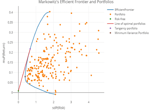
Figure 12. Table of Efficient Frontier by Shrunk Covariance Matrix with 200 bonds-IG

V. Findings and Conclusion

● First of all, Covariance Matrix is a way to quantify risks of securities.

● Second, Sample covariance matrix is not good enough to evaluate the risk, it causes bias and has high potential risk; and the CVm will be non-singular and cannot be inverted when the portfolio contains too many assets.

● Third, we do not obtain sufficient data for shrinkage estimation. In the future, we plan to try to conduct Shrunk Covariance Matrix by weekly data instead of monthly data.

Moreover, we explored weighted Sample Covariance matrix performed better for both High yield and Investment grade datasets. Both of them have small Mean Absolute Error based on our result.

Furthermore, we recommend that Weighted CVm would be suitable for small and non-specific time period data, however, shrinkage CVm would conduct better results for larger and more specific time period data.

Based on the data which is provided by Principal for now; we believe that the weighted Sample Covariance matrix is better than Sample covariance Matrix and Shrinkage Covariance Matrix. However, the shrinkage covariance matrix could be better when the data is more frequent than monthly data.

VI. Future Research

The data we used are not sufficient. For example, if we could use the full dataset such as 2011-2018 and all the bonds are on the similar maturity or use weekly data instead of monthly data to build samples, then perhaps the shrinkage covariance matrix might have performed better compared to other models. Moreover, try to use factor base analysis as target matrix for shrinkage estimation. This could provide more accurate results when we shrunk the outlier to the target mean and could reduce the model risk.

Secondly, we do suggest that research on Joint Mean-Covariance Modeling of Longitudinal Data (Pan & Pan, 2017). This method perhaps could be another way to estimate the Covariance Matrix. We believe that this model could solve the problem of the complicity in building a fixed income portfolio. For instance, we could use this method to estimate the excess return and use this predictive excess return to estimate the covariance matrix.

Finally, based on our research, sample covariance matrix and weighted sample covariance matrix does not work on a portfolio containing 100 assets. As a result, we suggest using real portfolio to back test the weighted covariance matrix and Shrinkage covariance matrix then establish the Sharpe Ratio in order to compare the result. This could give produce a better estimation of covariance matrix. Therefore, we suggest using weighted sample covariance matrix on small portfolio but use shrinkage covariance matrix on a large portfolio.

Appendix

Literature Review

1. A Comparison of Estimation Techniques for the Covariance Matrix in a Fixed-Income Framework

In this paper, Marco Neffelli and Marina Resta compared and estimated Shrinkage (SH), the Nonlinear Shrinkage (NSH), the Minimum Covariance Determinant (MCD) and the Minimum Regularized Covariance Determinant (MRCD) estimators with Sample Covariance Matrix (SCV) by using used Principal Component Analysis (PCA) and a robust approach, which is, LS hedging approach. According to the results of LS method, MCD and SCV estimators are the first two fastest factors to reach 99% threshold of explained variance. In addition, based on PCA approach, earlier three components of increased maturities by the sensitivity of changes in interest rate of MCD, SCV and NSH have a good performance, this result is similar with the LS. In conclusion, PCA approach is more powerful in financial products estimation, and MCD is better than the other methodologies.

2. MFE8812 Bond Portfolio Management / Investment Strategies

The paper explains the challenges of managing portfolios to match index returns, Straightforward replication for smaller portfolios would necessitate buying odd lots and lead to overwhelming transaction cost. an alternative approach, known as optimization or sampling, seeks to reproduce the overall attributes of the index with limited number of issues. The paper explains three basic approaches to index replication other than Straightforward replication:

● Stratified Sampling

● Tracking-error minimization

● Factor-based replication

3. Improved estimation of the covariance matrix of stock returns with an application to portfolio selection

This paper points out using shrinkage to the Improve estimation of the covariance matrix of stock returns. They propose to estimate the covariance matrix of stock returns by an optimally weighted average of two existing estimators: the sample covariance matrix and single-index covariance matrix. The crux of the method is to shrink the unbiased but very variable sample covariance matrix towards the biased but less variable single-index model covariance matrix and to system obtain a more efficient estimator. Therefore, in our article, we also can use this method to improve estimation of the covariance matrix of fixed-income.

4. Honey, I Shrunk the Sample Covariance Matrix

This paper points out that the sample covariance matrix cannot be used directly to portfolio optimization. Due to the volatility and diversity of the data, direct use that can seriously affect the estimates of the mean and variance, resulting in large errors. Therefore, this paper proposes that they need to use the method of shrinkage to construct the covariance matrix. However, optimal shrinkage intensity is the biggest challenge in building accurate covariance matrices. The article uses stock market data as an example to illustrate how to shrink and reduce errors. Therefore, in our paper, we can improve the search for the shrinkage target and shrinkage intensity according to the formula of this paper, thereby achieving a reduction in error.

Second: Since our data is large, if we apply sample covariance matrix as it is, the chance of getting lot of error is high. Which means most extreme coefficients in the matrix will tend to take extreme values because it contains extreme amount of error. This is why in this paper they proposed new formulae for estimating the covariance matrix for returns. The crux of the method is that those estimated coefficients in the sample covariance matrix that are extremely high tend to contain a lot of positive error and therefore need to be pulled downwards to compensate for that. Similarly, for the negative error pull them to upwards. This is called as shrinkage of the extremes towards the center. Fixing this shrinkage will solve the problem. The Paper derives the formula for reducing the shrinkage.

5. Size Matters: Optimal Calibration of Shrinkage Estimators for Portfolio Selection

The author indicates that they used different Shrinkage for portfolio selection. The first is shrinking the mean of assets return and the second is the CVm’s assets return are weight the portfolio directly. However, they provide a new calibration for shrinkage estimator of covariance matrix that take condition number into account. Autor clearly justify that the problem of CVm in portfolio, As the result, they provide a new solution which is using expected quadratic loss and condition number in order to show the corresponding shrinkage intensity could be obtain numerically. Therefore, the result shows that this model is better for mid and large dataset.

References

1. Martellini, L., Priaulet, P., & Priaulet, S. (2003). Investment Strategies. In Fixed-income securities : valuation, risk management, and portfolio strategies (pp. 213-316). Chichester, England ;: Wiley

2. Ledoit, O., & Wolf, M. N. (2003). Honey, I Shrunk the Sample Covariance Matrix. SSRN Electronic Journal. doi:10.2139/ssrn.433840

3. Demiguel, V., Martin-Utrera, A., & Nogales, F. J. (2011). Size Matters: Optimal Calibration of Shrinkage Estimators for Portfolio Selection. SSRN Electronic Journal. doi:10.2139/ssrn.1891847

4. Ledoit, O., & Wolf, M. (2003). Improved estimation of the covariance matrix of stock returns with an application to portfolio selection. Journal of Empirical Finance,10(5), 603-621. doi:10.1016/s0927-5398(03)00007-0

5. Stephanie. (2016, October, 23). Shrinkage Estimator: Definition, Examples.

Retrieved from https://www.statisticshowto.datasciencecentral.com/shrinkage-estimator/

6. Miller, T. (2019, March 22). What Is Modern Portfolio Theory (MPT) and Why Is It Important? Retrieved from https://www.thestreet.com/investing/modern-portfolio-theory-14903955

7. Karoui, N. E. (2010). High-dimensionality effects in the Markowitz problem and other quadratic programs with linear constraints: Risk underestimation. The Annals of Statistics,38(6), 3487-3566. doi:10.1214/10-aos795. Retrieved from https://projecteuclid.org/download/pdfview_1/euclid.aos/1291126965

8. Elton, E. J., & Gruber, M. J. (1997). Modern portfolio theory, 1950 to date. Journal of Banking & Finance,21(11-12), 1743-1759. doi:10.1016/s0378-4266(97)00048-4

9. Chen, J. (2019, April 27). The Benefits and Risks of Fixed Income Products. Retrieved from https://www.investopedia.com/terms/f/fixedincome.asp

10. GRACE-MARTIN, K. (2018, December 09). Covariance Matrices, Covariance Structures, and Bears, Oh My! Retrieved from https://www.theanalysisfactor.com/covariance-matrices/

11. Weighted Cov (n.d.). Retrieved from https://www2.microstrategy.com/producthelp/10.8/FunctionsRef/Content/FuncRef/WeightedCov__weighted_covariance_.htm

12. Chen, J. (2019, April 17). Modern Portfolio Theory (MPT). Retrieved from https://www.investopedia.com/terms/m/modernportfoliotheory.asp

13. Neffelli, M., & Resta, M. (2018). A Comparison of Estimation Techniques for the Covariance Matrix in a Fixed-Income Framework. New Methods in Fixed Income Modeling Contributions to Management Science,99-115. doi:10.1007/978-3-319-95285-7_6

14. Pan, J., & Pan, Y. (2017). Jmcm: An R Package for Joint Mean-Covariance Modeling of Longitudinal Data. Journal of Statistical Software,82(9). doi:10.18637/jss.v082.i09